Visualization with Rerun

Full source code

Rosia integrates with Rerun for visualizing node data over time. Rerun provides an interactive viewer that plots data against both logical and physical time.

Logging with log.rerun()

from rosia import log
import rerun as rr

Use log.rerun() to log any Rerun archetype from within a node:

log.rerun(archetype, rerun_subpath="...")

• archetype — any Rerun component (rr.Points3D, rr.LineStrips3D, rr.Image, rr.TextLog, etc.).
• rerun_subpath — controls where it appears in the Rerun entity tree.

Data is indexed by both logical time and physical time, so you can scrub through the timeline in either mode.

Enabling Rerun

Pass a RerunConfig to app.execute() to enable Rerun logging:

from rosia.config import RerunConfig

app.execute(rerun_config=RerunConfig())

Optionally, pass a Rerun blueprint to configure the viewer layout:

import rerun.blueprint as rrb

app.execute(
    rerun_config=RerunConfig(
        blueprint=rrb.Blueprint(rrb.Spatial3DView(origin="/"))
    )
)

Enabling Tracing

Pass trace=True to app.execute() to enable automatic tracing. When tracing is enabled:

• All input port values are automatically logged to Rerun on each reaction.
• Text log messages from log.info(...), log.debug(...), etc. appear in the Rerun timeline.

app.execute(trace=True, rerun_config=RerunConfig())

Full Example: Bouncing Ball

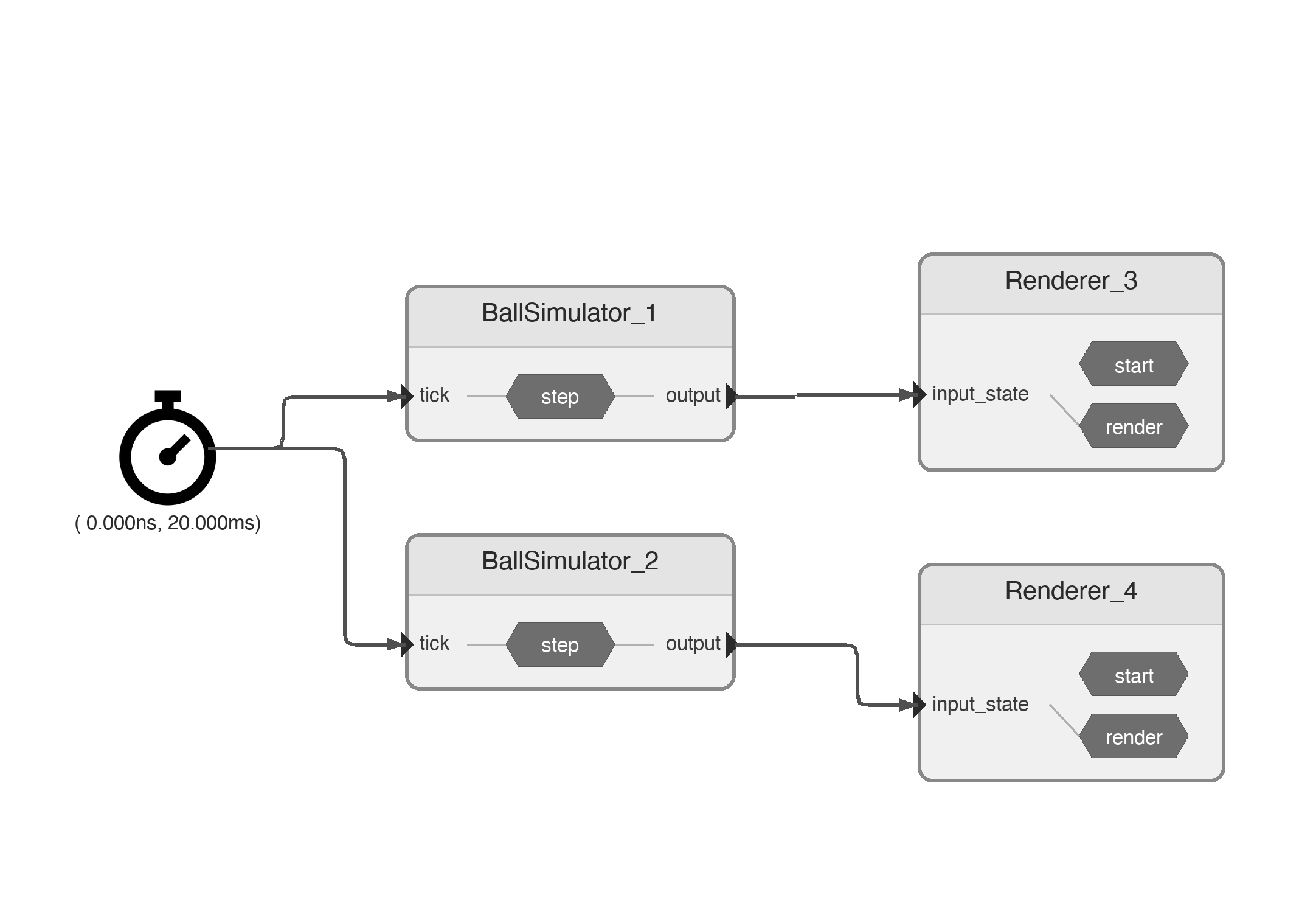
This example simulates two bouncing balls and visualizes them with Rerun.

Pipeline

Data

import numpy as np
import rerun as rr

class BallState:
    def __init__(self, position: np.ndarray, velocity: np.ndarray, color: list[int]):
        self.position = position
        self.velocity = velocity
        self.color = color

Nodes

from rosia import InputPort, OutputPort, reaction, Node, Application, request_shutdown, log
from rosia.config import RerunConfig
from rosia.time import Timer, Time, s, ms
import rerun.blueprint as rrb


@Node
class BallSimulator:
    tick = InputPort[Time]()
    output = OutputPort[BallState]()

    def __init__(self, initial_position, initial_velocity, gravity=-9.81,
                 restitution=0.85, dt=0.02, max_ticks=100, color=[255, 100, 50]):
        self.position = np.array(initial_position, dtype=float)
        self.velocity = np.array(initial_velocity, dtype=float)
        self.gravity = gravity
        self.restitution = restitution
        self.dt = dt
        self.max_ticks = max_ticks
        self.tick_count = 0
        self.color = color

    @reaction([tick])
    def step(self):
        self.velocity[2] += self.gravity * self.dt
        self.position += self.velocity * self.dt
        if self.position[2] <= 0.0:
            self.position[2] = -self.position[2]
            self.velocity[2] = -self.velocity[2] * self.restitution
        self.output(BallState(self.position, self.velocity, self.color))
        self.tick_count += 1
        if self.tick_count >= self.max_ticks:
            request_shutdown()


@Node
class Renderer:
    input_state = InputPort[BallState]()

    def start(self):
        # Log static ground plane grid
        lines = []
        for i in np.linspace(-5, 15, 21):
            lines.append([[i, -5, 0], [i, 15, 0]])
            lines.append([[-5, i, 0], [15, i, 0]])
        log.rerun(
            rr.LineStrips3D(lines, colors=[[200, 200, 200]]),
            rerun_subpath="ground",
        )

    @reaction([input_state])
    def render(self):
        state = self.input_state
        log.info(f"ball {state}")
        log.rerun(
            rr.Points3D(
                [state.position],
                radii=[0.3],
                colors=[state.color],
            ),
            rerun_subpath="ball",
        )

Wiring

app = Application()
timer = app.create_node(Timer(interval=20 * ms, offset=0 * s))
sim1 = app.create_node(BallSimulator(initial_position=(0, 0, 5), initial_velocity=(2, 1.5, 0), color=[255, 100, 50]))
sim2 = app.create_node(BallSimulator(initial_position=(0, 3, 5), initial_velocity=(2, 1.5, 0), color=[50, 150, 255]))
renderer1 = app.create_node(Renderer())
renderer2 = app.create_node(Renderer())

timer.output_timer >>= sim1.tick
timer.output_timer >>= sim2.tick
sim1.output >>= renderer1.input_state
sim2.output >>= renderer2.input_state

app.execute(
    rerun_config=RerunConfig(
        blueprint=rrb.Blueprint(rrb.Horizontal(rrb.Spatial3DView(origin="/")))
    )
)

Run this and the Rerun viewer opens with:

• A 3D view showing two balls bouncing on a grid
• A timeline scrubber indexed by logical time and physical time
• Text logs from each node